
Problem
Graphical Interface
Finding Optimal Decisions
Considering Sub-Optimal Decisions
Filters
Decision Pool
Integrated Optimization Objective
Decision Navigation Buttons
Underlying Decision Model
We need to help a manufacturer decide how much of each demanded product should be produced internally and how much should be sourced from outside. Whether a product is made inside or outside, it has an associated cost. A product can consume a given amount of internal resources that have limited capacities. The general objective is to minimize the total production cost while ensuring the company meets the demand exactly or with a certain tolerance. This DMCommunity’s challenge provides the following data samples with products, resources, and capacity requirements:
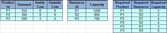
The manufacturer wants to consider various production decisions to choose the most suitable ones based on the long-term resource availability and uncertain future demand. This sample demonstrates how OpenRules Decision Playground can be used to find the best production decision.
The proper decision model is implemented as a simple project, “InsideOutsideProduction” coming with OpenRules Rule Solver. You can find its implementation at the end of this page. Now you may use Decision Playground to generate various production decisions using the same decision model.
Click on “InsideOutsideProduction/play.bat” to start Decision Playground. Decision Playground can be used with different underlying open-source or commercial Constraint Solvers or Linear/MIP Solvers as defined by the environment variable SOLVER in the launch file “play.bat”:
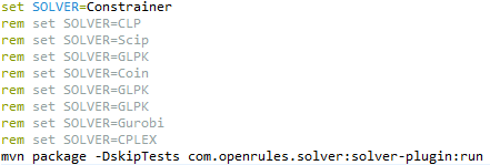
Let’s start with the constraint solver “Constrainer”.
Here is your Playground’s view after you click on “New Request” to select a JSON file with input data:
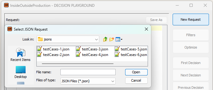
The proper JSON files, such as “testCases-1.json,” were generated based on the test cases in Excel during the testing of the decision model. Still, you may also create a JSON request manually or get it from your production system.
Then you may click on “Optimize” to get the following Decision Playground’s view:
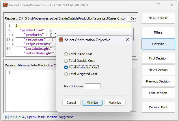
Let’s say you first want to minimize the Total Production Cost. You can select “Total Production Cost” as your optimization objective and click “Minimize”. The Playground will run the decision model to produce the proper optimal decision. With the underlying constraint solver, the search will take around 1 minute. When the optimal decision is found, the Playground will show the following dialog that includes the number of the found solution:
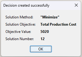
You may analyze the found optimal decision in the bottom part of the Playground screen:
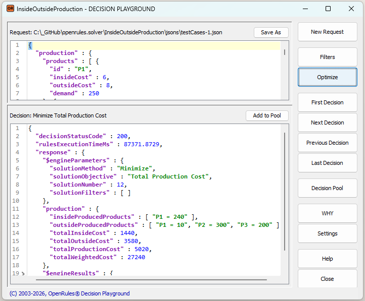
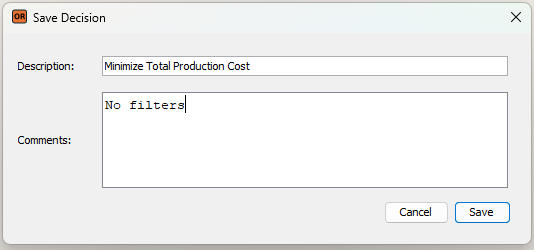
This decision indicates which products, and in what quantities, should be produced internally versus externally to achieve the minimum possible total production cost of $5,020. You may memorize this decision in the Decision Pool by selecting “Add to Pool”:
Probably you would like to produce more products internally, even if the total production cost would go slightly up. To do this, you may choose a different optimization criterion:
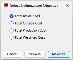
You will receive the following decision, which you may also add to the Decision Pool:
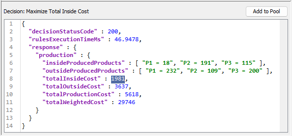
So, you may produce internally 18 products P1, 191 products P2, and 115 products P3 to achieve the maximum possible inside cost of $1,981. However, using this decision, your total production cost will grow from $5,020 to $5,618. You may define filters to find a trade-off decision.
Considering Sub-Optimal Decisions
If you are not satisfied with the optimal decision, they can request alternative solutions by limiting “Max Solutions” to a number smaller than the found optimal solution, e.g. 8:
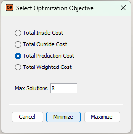
In this case, the Playground will show you the solution #8 by stopping short on the way to the optimal solution #12:
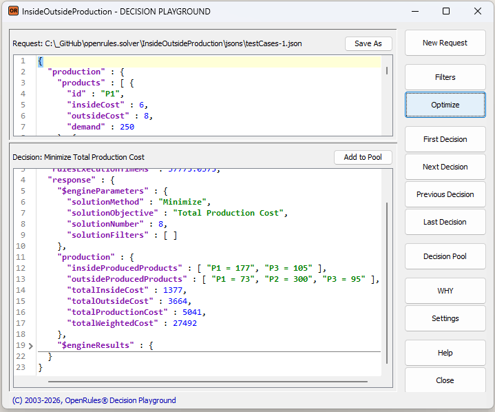
This alternative solution may be less optimal but more practical given your current business conditions and constraints. For example, in this case the Total Production Cost of $5,041 is slightly higher than the optimal cost of $5,020 but more products will be produced internally.
Another way to finding alternative decisions that trade optimality for better alignment with your current business conditions is the use of filters. The button “Filters” allows you quickly add additional constraints to tune the decision model to the reality of a particular decisioning situation.
For example, in this model you probably want to increase the total inside cost inside the interval [$1,440; $1,981] while still minimizing the total production cost. You may limit the total inside cost to be larger than $1,700 using the following Filter:
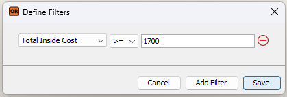
Save this filter and choose again “Optimize” to minimize the Total Production Cost. You will receive a new decision:
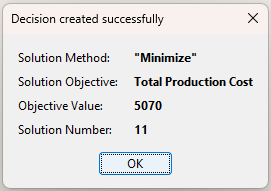
described as below:
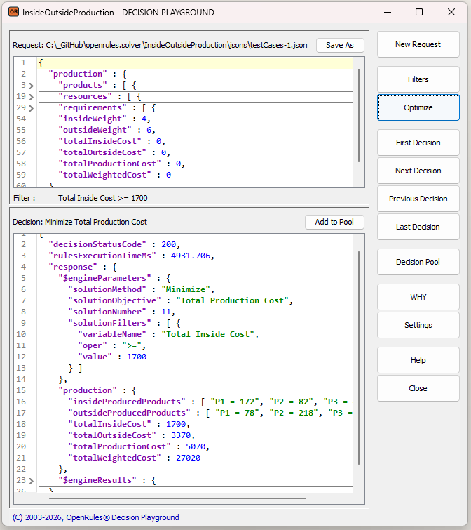
This decision will increase the total production cost only by $50, but it would produce more products internally. So, instead of the threshold of $1,700 we may try $1,800 by modifying the filter. Here is the resulting decision:
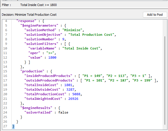
This decision looks even better. You may try two filters:
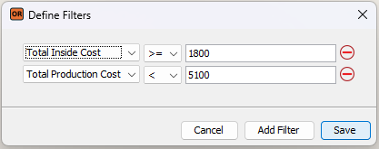
and again maximize the Total Inside Cost:
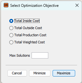
You will receive an even better decision:
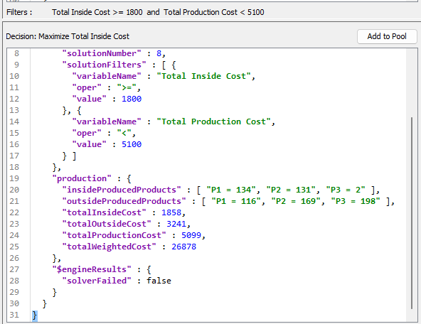
Let’s save this decision in Decision Pool as well.
Click on the button “Decision Pool” to compare all the saved decisions we received so far:
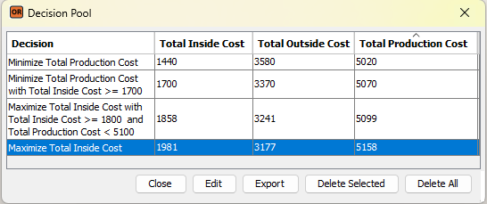
You can continue experimenting with different filters and optimization objectives to obtain the decisions that best suit your situation.
Integrated Optimization Objective
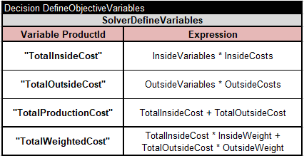
This decision model defines one more optimization goal called “Total Weighted Cost“, which is defined by the following formula:
totalInsideCost*insideWeight + totalOutsideCost*outsideWeight
In our request, we may define insideWeight=3 and outsideWeight=6. Then, without any filters, we may use the following optimization criterion:
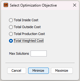
It will give us the following decision:
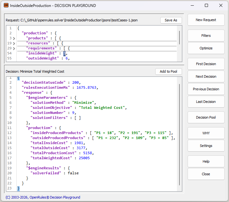
You can save this decision and compare all found decisions by looking inside the Decision Pool:
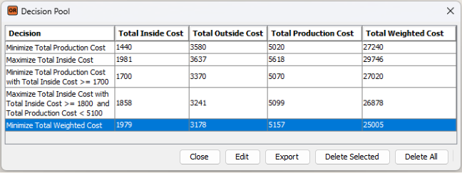
Inside the Pool, you can visually compare different Decision-Candidates, sort them by different KPIs, and choose the Decision-Champion that best fits the current situation. This decision can then be exported for further use and future Decision Tracing.
When the number of possible decisions is relatively small, you can browse all available options using the buttons “First Decision”, “Next Decision”, “Previous Decision”, and “Last Decision” to choose the “best” one without invoking any optimization. For example, after a click on “First Decision” you will receive:
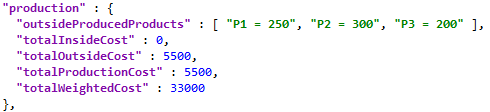
A click on “Next Decision” will produce:
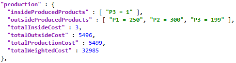
A click on “Last Decision” may work too long as there are too many possible solutions. So, you may limit to total number of considered solution say to 100 by clicking on “Settings” and defining “Max Solutions” as 100:
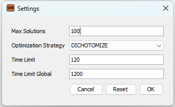
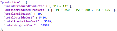
Alternatively or additionally you may set Time Limit for the search of one decision (here it is set to 120 seconds) and Time Limit Global for the entire search (here it is set to 1200 seconds). If you click on “Last Decision” now, you will quickly receive the following decision:
You may use these decision navigation buttons along with filters.
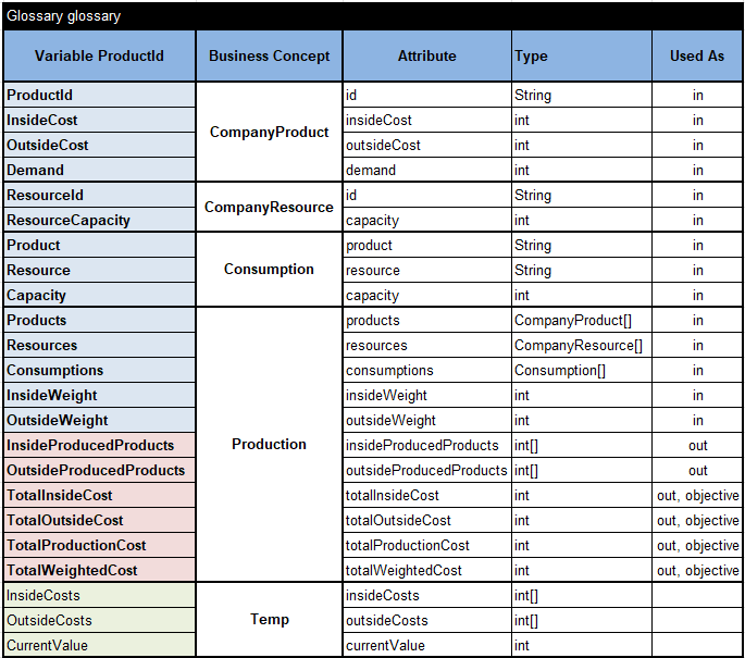
This example is based on the decision model “InsideOutsideProduction” located in “openrules.solver/ADVANCED”. Here is the Glossary:
Here are two main methods, “Define” and “Solve”, that are pretty common for decision models utilizing Rule Solver:
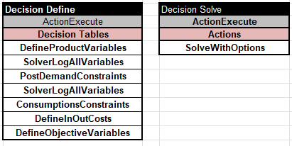
The table “DefineProductVariables” for each product P in the input array “Products” defines the proper constrained decision variables with names like “InsideP1” or “OutsideP2” with possible values from 0 to the Demand of this particular product:
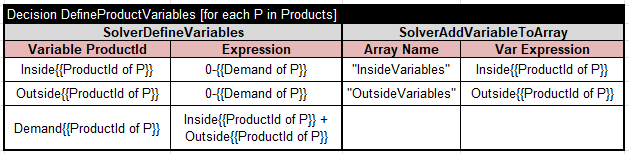
It also defines the demand variables like “DemandP1” that should be equal to the sum of variables “InsideP1” and “OutsideP1”. It adds the product variables to the arrays “InsideVariables” and “OutsideVariables” that will be needed to specify optimization objectives.
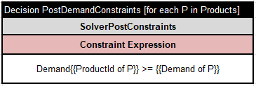
The table “PostDemandConstraints” for each product P in the input array “Products” posts a constraint that states that the proper demand decision variable should not be less than the required demand of this product:
The table “ConsumptionConstraints”
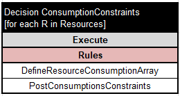
for each resource R in the array “Resources” does the following. First, it executes this table to define an array with all resource consumption variables for each consumption in the array “Consumptions”:

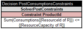
Then it executes this table to post the main consumption constraint for each resource:
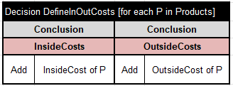
To define optimization objectives, first we need to use temporary arrays “InsideCosts” and “Outside Costs” that can be easily filled out by the regular OpenRules decision table “DefineInOutCosts”:
The following table defines all optimization objectives as new constrained decision variables:
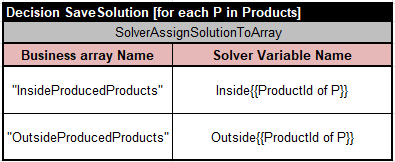
The table “Solve” relies on the standard solving method “SolveWithOptions”. When a solution is found, this method automatically invokes the method “SaveSolution” if it exists. This decision model saves every solution using the following table:
If you make changes to the decision model, you need to restart Decision Playground to see how they affect the generated decisions.